import matplotlib.pyplot as plt
import torch
import torch.distributions as dist
from random import random
Introduction to Probability Theory
Random Variables
A random variable $X$ is a mapping from a probability space to a state space.
It is easier to think of random variables as distributions on the state space.
Discrete Random Variables
Discrete random variables has only a finite or countably infinite number of outcomes.
For instance, the natural numbers are countably infinite.
The distribution of a discrete random variable can be fully specified by a probability mass function $p_X$.
$$P(X=x) = p_X(x)$$
Example 1:
A binomial variable models the number of successes in a sequence of $n$ independent experiments, each having a success probability of $p$.
Thus, the outcomes are $\{0,...,n\}$ and the probability mass function can be written as
$$P(X = k) = p_X(k) = \binom{n}{k} p^k (1-p)^{n-k}$$
n = 10
p = 0.25
d = dist.Binomial(n, p)
outcomes = torch.arange(0,10+1)
probs = d.log_prob(outcomes).exp() # computes probability mass function
plt.bar(outcomes, probs)
plt.xlabel("Outcomes")
plt.ylabel("Probability")
plt.show()
We can check that the probability mass function indeed gives the correct probabilities, by running a simulation.
def sample_binomial(n,p):
    n_success = 0
    for _ in range(n):
        success = random() < p
        n_success += success
    return n_success

sample = torch.tensor([sample_binomial(n,p) for _ in range(10000)])
est_probs = [(sample == k).float().mean() for k in outcomes]
plt.bar(outcomes, probs)
plt.bar(outcomes + 0.2, est_probs, alpha=0.75)
plt.xlabel("Outcomes")
plt.ylabel("Probability")
plt.show()
Example 2:
An example for a discrete random variable with infinite possible outcomes is a Geometric distribution.
The geometric distribution gives the probability that the first occurance of success requires $k$ fails of independent trials.
$$p_X(k) = (1-p)^k p$$
p = 0.2
d = dist.Geometric(p)
outcomes = torch.arange(0,25)
probs = d.log_prob(outcomes).exp()
plt.bar(outcomes, probs)
plt.xlabel("Outcomes")
plt.ylabel("Probability")
plt.show()
def sample_geometric(p):
    n_fails = 0
    while True:
        success = random() < p
        if success == 0:
            n_fails += 1
        else:
            break
    return n_fails


sample = torch.tensor([sample_geometric(p) for _ in range(10000)])
est_probs = [(sample == k).float().mean() for k in outcomes]
plt.bar(outcomes, probs)
plt.bar(outcomes + 0.2, est_probs, alpha=0.75)
plt.xlabel("Outcomes")
plt.ylabel("Probability")
plt.show()
Example 3:
Another important discrete distribution is the Categorical distribution.
Here, we specifiy a probability vector $p_k$ such that $\sum_{k=1}^n p_k = 1$.
It can be interpreted as an experiment that falls into category $k$ with probability $p_k$.
$$p_X(k) = p_k$$
For instance, a dice follows a categorical distribution with $p=[\frac{1}{6},\frac{1}{6},\frac{1}{6},\frac{1}{6},\frac{1}{6},\frac{1}{6}]$
Probability Mass Function
The probability mass function fully describes the distribution of $X$ as we can compute the probability of any set of outcomes $A$ simply as sum: $$P(X \in A) = \sum_{k \in A} p_X(k)$$
# Compute probability that number of failures is greater than or equal to 2 and less than or equal to 5
p = 0.2
d = dist.Geometric(p)

outcomes = torch.arange(0,25)
probs = d.log_prob(outcomes).exp()
plt.bar(outcomes, probs, alpha=0.1)
plt.xlabel("Outcomes")
plt.ylabel("Probability")

a = 2
b = 5
selected_outcomes = torch.arange(a,b+1)
plt.bar(selected_outcomes, d.log_prob(selected_outcomes).exp(), color="tab:blue")
plt.show()

d.log_prob(selected_outcomes).exp().sum()
tensor(0.3779)
# the probability of taking any possible outcome is of course 1.
n = 10
p = 0.25
d = dist.Binomial(n, p)
outcomes = torch.arange(0,10+1)
d.log_prob(outcomes).exp().sum()
tensor(1.0000)
Continuous Random Variables
Continuous random variables have distribution on the real numbers or an interval on the real line.
They can be defined by a probability density function $f_X$.
The probability of any interval can be computed with an integral:
$$P(a \le X \le b) = \int_{a}^b f_X(x) dx$$
Or more for any subset of outcomes with the generalised (Lebesgue) integral:
$$P(X \in A) = \int_A f_X(x) dx$$
Example 1:
Normal distribution with mean $\mu$ and standard deviation $\sigma$:
$$p_X(x) = \frac{1}{\sqrt{2\pi\sigma^2}}\exp\left(-\frac{(x-\mu)^2}{2\sigma^2}\right)$$
mu = 1
sigma = 0.5
d = dist.Normal(mu, sigma)
outcomes = torch.linspace(-5,5,200)
probs = d.log_prob(outcomes).exp() # computes probability density function
plt.plot(outcomes, probs)
plt.xlabel("X")
plt.ylabel("Probability")
plt.show()
Example 2:
A beta distribution is defined on $[0,1]$ and can be used to model unknown probabilities.
$$p_X(x) = \frac{1}{B(\alpha, \beta)} x^{\alpha-1} (1-x)^{\beta-1}$$
alpha = 5
beta = 2
d = dist.Beta(alpha,beta)
outcomes = torch.linspace(0,1,200)
probs = d.log_prob(outcomes).exp() # computes probability density function
plt.plot(outcomes, probs)
plt.xlabel("X")
plt.ylabel("Probability")
plt.show()
Probability Density Function
Again, the probability density function fully defines the distribution of a continuous random variable.
a = 0.6
b = 0.9

outcomes = torch.linspace(0,1,500)
probs = d.log_prob(outcomes).exp()
plt.plot(outcomes, probs)

interval = torch.linspace(a,b,500)
interval_probs = d.log_prob(interval).exp()
plt.fill_between(interval, interval_probs)

plt.xlabel("X")
plt.ylabel("Probability")
plt.show()

# numerical integration
print("probability of interval:", torch.trapz(interval_probs, interval).item())
probability of interval: 0.6524544358253479
# integral over whole outcome space is one
torch.trapz(probs, outcomes)
tensor(1.0000)
Expected Value, Variance, and Mode
The expected value (mean) of a random variable with a finite number of outcomes is a weighted average of all possible outcomes.
$$\mathbb{E}(X) = \sum_{x} x \cdot p_X(x)$$
In the case of continuous variables, the expectation is generalised with integration.
$$\mathbb{E}(X) = \int x \cdot f_X(x)\;dx$$
If we take a large sample of independently generated outcomes, then the arithmetic mean is close to the expected value.
The variance is the expected squared deviation from the mean.
$$\text{Var}(X) = \mathbb{E}[(X-\mathbb{E}(X))^2]$$
The mode of a random variable is the outcome with highest probability.
It maximises the probability mass/density function.
a = 4
b = 2
d = dist.Beta(a,b)
ps = torch.linspace(0,1,500)
density = d.log_prob(ps).exp()
plt.plot(ps, density)
plt.vlines(d.mode, 0., d.log_prob(d.mode).exp(), label="mode", color="tab:green")
plt.vlines(d.mean, 0., d.log_prob(d.mean).exp(), label="mean", color="tab:orange")
m_minus_s = d.mean - torch.sqrt(d.variance)
m_plus_s = d.mean + torch.sqrt(d.variance)
plt.vlines([m_minus_s, m_plus_s], 0., [d.log_prob(m_minus_s).exp(), d.log_prob(m_plus_s).exp()], label="mean +/- sqrt(variance)", color="tab:red")
plt.legend()
plt.show()
d.mean, torch.trapz(ps * density, ps)
(tensor(0.6667), tensor(0.6667))
d.variance, torch.trapz((ps - d.mean)**2 * density, ps)
(tensor(0.0317), tensor(0.0317))
d.mode, ps[density.argmax()]
(tensor(0.7500), tensor(0.7495))
Monte Carlo Method
At this point we should justify, why simulation-based methods work.
The law of large numbers says that for an sequence of independent and identical distributed (iid) random variables $X_i$ (with finite variance or integrable), then
$$\frac{1}{n}\sum_{i=1}^n X_i \to \mu \quad \text{as}\; n \to \infty,$$
where $\mu$ is the expected value of $X_i$.
This implies that a with large enough sample the histogram follows the density function.
N = 100000

a = 4
b = 2
d = dist.Beta(a,b)
ps = torch.linspace(0,1,100)

sample = d.sample((N,))
plt.hist(sample, density=True, bins=ps)
plt.plot(ps, d.log_prob(ps).exp())
plt.show()

sample.mean(), d.mean
(tensor(0.6667), tensor(0.6667))
Joint Probability Distribution
Given two random variables $X$, $Y$, the joint probability distribution is the corresponding probability distribution on all possible pairs of outputs, $P(X,Y)$.
In the simplest case, $X$ and $Y$ are independent and we have $P(X \in A,Y \in B) = P(X \in A) P(Y \in B)$.
The multi-variate random variable $(X,Y)$ is distributed according to $P(X,Y)$.
For discrete variabels, we can define a joint probability mass function $p_{XY}(x,y)$:
$$P(X \in A,Y \in B) = \sum_{x \in A} \sum_{y \in B} p_{XY}(x,y)$$
For continuous variabels, we can define a joint probability density function $f_{XY}(x,y)$:
$$P(X \in A,Y \in B) = \int_{B} \int_{A} f_{XY}(x,y)dx dy$$
Example 1:
Consider two independent experiments. The first has success probability 0.3, the second one 0.8.
experiment_1 = dist.Bernoulli(0.3)
experiment_1_outcomes = [0.,1.]
experiment_2 = dist.Bernoulli(0.8)
experiment_2_outcomes = [0.,1.]

joint = torch.zeros((len(experiment_1_outcomes), len(experiment_2_outcomes)))
for i, o1 in enumerate(torch.tensor(experiment_1_outcomes)):
    for j, o2 in enumerate(torch.tensor(experiment_2_outcomes)):
        joint[i,j] = experiment_1.log_prob(o1).exp() * experiment_2.log_prob(o2).exp()

plt.yticks(experiment_1_outcomes, experiment_1_outcomes)
plt.xticks(experiment_2_outcomes, experiment_2_outcomes)
for i in range(joint.shape[0]):
    for j in range(joint.shape[1]):
        color = "white" if joint[i,j] < 0.5 else "black"
        plt.text(j,i, f"{joint[i,j].item():.2f}", ha="center", va="center", color=color)

plt.ylabel("Experiment 1")
plt.xlabel("Experiment 2")
plt.imshow(joint)
plt.show()
We can see that the probability for failing in experiment 1 and succeeding in experiment 2 is highest.
# the joint sums to 1
joint.sum()
tensor(1.)
Example 2:
Suppose, we have 5 urns with a total of 10 balls.
In the urns are 0, 2, 4, 6, and 8 red balls respectively, the rest are black.
We choose an urn at random and draw five balls, each time putting the ball back in the urn.
The number of drawn red balls is dependent on the number of balls in the chosen urn.
In this case, the joint may be written as $P(X,Y) = P(Y|X) P(X)$, where $X$ is the random variable for choosing the urn, and $Y$ is the random variable for drawing the balls. More details later.
urn = dist.Categorical(torch.tensor([0.2,0.2,0.2,0.2,0.2]))
n_urns = 5
red_balls = [0,2,4,6,8]
total_balls = 10
n_draws = 5
urn_joint = torch.zeros((n_draws+1,n_urns))
for i in range(n_draws+1): # i ... number of red balls drawn
    for j in range(n_urns): # j ... chosen urn
        category = torch.tensor(j)
        p = red_balls[j] / total_balls
        ball_draws = dist.Binomial(n_draws,p)
        n_red_balls = torch.tensor(i)
        urn_joint[i,j] = urn.log_prob(category).exp() * ball_draws.log_prob(n_red_balls).exp()


for i in range(urn_joint.shape[0]):
    for j in range(urn_joint.shape[1]):
        color = "white" if urn_joint[i,j] < 0.1 else "black"
        plt.text(j,i, f"{urn_joint[i,j].item():.2f}", ha="center", va="center", color=color)

plt.xlabel("Chosen urn")
plt.ylabel("Number of red balls drawn")

plt.imshow(urn_joint)
plt.show()
Example 3:
The joint distribution of two continous variables forms a 2D surface.
mu_1 = 1.
sigma_1 = 2.
mu_2 = 0.
sigma_2 = 1.

dist_x = dist.Normal(mu_1, sigma_1)
dist_y = dist.Normal(mu_2, sigma_2)

xs = torch.linspace(-4,6,200)
ys = torch.linspace(-5,5,200)

joint = torch.zeros((len(ys), len(xs)))

for j, x in enumerate(xs):
    for i, y in enumerate(ys):
        joint[j,i] = dist_x.log_prob(x).exp() * dist_y.log_prob(y).exp()

from matplotlib import cm

fig, ax = plt.subplots(subplot_kw={"projection": "3d"})
X, Y = torch.meshgrid(xs, ys, indexing="ij")
ax.plot_surface(X, Y, joint, cmap=cm.coolwarm)
ax.set_title("Joint of two Normals")
ax.set_xlabel("X")
ax.set_ylabel("Y")
plt.show()
This leads to multivariate normal distributions.
mu_1 = 1.
sigma_1 = 2.
mu_2 = 0.
sigma_2 = 1.

xs = torch.linspace(-4,6,200)
ys = torch.linspace(-5,5,200)

joint = torch.zeros((len(ys), len(xs)))

joint_mv = torch.zeros((len(ys), len(xs)))
mv_dist = dist.MultivariateNormal(torch.tensor([mu_1,mu_2]), torch.tensor([[sigma_1**2, 1.], [1., sigma_2**2]]))

for j, x in enumerate(xs):
    for i, y in enumerate(ys):
        mu_cond = mu_2 + (x - mu_1) / sigma_1**2
        sigma_cond = torch.sqrt(torch.tensor(sigma_2**2 - 1/sigma_1**2))
        dist_x = dist.Normal(mu_1, sigma_1)
        dist_y = dist.Normal(mu_cond, sigma_cond)
        joint[j,i] = dist_x.log_prob(x).exp() * dist_y.log_prob(y).exp()

        joint_mv[j,i] = mv_dist.log_prob(torch.tensor([x,y])).exp()


from matplotlib import cm

fig, ax = plt.subplots(1,2,subplot_kw={"projection": "3d"})
X, Y = torch.meshgrid(xs, ys, indexing="ij")
ax[0].plot_surface(X, Y, joint, cmap=cm.coolwarm)
ax[0].set_title("Joint of two Normals")
ax[0].set_xlabel("X")
ax[0].set_ylabel("Y")
ax[1].plot_surface(X, Y, joint_mv, cmap=cm.coolwarm)
ax[1].set_title("Multi-variate Normal")
ax[1].set_xlabel("X")
ax[1].set_ylabel("Y")
plt.show()
(joint_mv - joint).abs().max()
tensor(2.9802e-08)
Marginal Distribution
For two random variables $X$ and $Y$ with joint distribution $P(X,Y)$, the marginal distribution gives the probabilities of one variable without reference to the other variable.
For two discrete variables this is achieved by "summing out" one variable: $$p_Y(y) = \sum_x p_{XY}(x,y)$$
For two continuous variables we have to "integrate out" one variable: $$f_Y(y) = \int f_{XY}(x,y) dx$$
With increasing number of random variables in the joint distribution, marginalisation is very expensive to compute (exponential): $$p_Y(y) = \sum_{x_1}\cdots \sum_{x_2} p_{XY}(x_1,\dots,x_n,y)$$
$$f_Y(y) = \int \cdots \int f_{XY}((x_1,\dots,x_n,y) dx_1 \cdots dx_n$$
Example
For two discrete random variables we can find the marginals, by computing row and column sums.
# For the urn model, the marignal probability of choosing an urn just tells us that we picked the urn at random
# It equals the column sum
for j in range(urn_joint.shape[1]):
    print(f"Prob. of picking urn {j}:", urn_joint[:,j].sum()) # sum out drawing balls
Prob. of picking urn 0: tensor(0.2000)
Prob. of picking urn 1: tensor(0.2000)
Prob. of picking urn 2: tensor(0.2000)
Prob. of picking urn 3: tensor(0.2000)
Prob. of picking urn 4: tensor(0.2000)
# More interestingly, we can compute the probability of drawing red balls
# without reference to the chosen urn
# It equals the row sum
for i in range(urn_joint.shape[0]):
    print(f"Prob. of drawing {i} red balls:", urn_joint[i,:].sum()) # sum out choosing urn
Prob. of drawing 0 red balls: tensor(0.2832)
Prob. of drawing 1 red balls: tensor(0.1504)
Prob. of drawing 2 red balls: tensor(0.1664)
Prob. of drawing 3 red balls: tensor(0.1664)
Prob. of drawing 4 red balls: tensor(0.1504)
Prob. of drawing 5 red balls: tensor(0.0832)
Conditional Probability
The conditional probability is a measure of the probability of an event $A$ occurring, given that another event $B$ has already occurred.
Mathematically, $$P(A|B) = \frac{P(A \cap B)}{P(B)}.$$
For two random variables $X$, $Y$ the conditional random variable $Y|X$ is given by
$$P(Y \in B | X \in A) = \frac{P(Y \in B, X \in A)}{P(X \in A)}. $$
Thus, for discrete variables
$$p_{Y|X}(y|x) = \frac{p_{XY}(x,y)}{p_{X}(x)} = \frac{p_{XY}(x,y)}{\sum_y p_{XY}(x, y)}$$
and for continuous variables
$$f_{Y|X}(y|x) = \frac{f_{XY}(x,y)}{f_{X}(x)} = \frac{f_{XY}(x,y)}{\int f_{XY}(x, y)dy}$$
Example 1
n_red_balls_drawn = 3

urn_joint_filtered = urn_joint[n_red_balls_drawn,:] # p(x=n_red_balls_drawn, y)
normalizer = urn_joint_filtered.sum() # P(x=n_red_balls_drawn)
urn_conditional = urn_joint_filtered / normalizer

for i in range(len(urn_conditional)):
    print(f"Prob. of having picked urn {i} given {n_red_balls_drawn} red balls drawn: {urn_conditional[i]:.2f}")
Prob. of having picked urn 0 given 3 red balls drawn: 0.00
Prob. of having picked urn 1 given 3 red balls drawn: 0.06
Prob. of having picked urn 2 given 3 red balls drawn: 0.28
Prob. of having picked urn 3 given 3 red balls drawn: 0.42
Prob. of having picked urn 4 given 3 red balls drawn: 0.25
We may also compute the conditional probability table.
It computes above distribution for every number of red balls drawn.
Note that the columns sum to one.
urn_conditional = urn_joint.T / urn_joint.T.sum(dim=0)

for i in range(urn_conditional.shape[0]):
    for j in range(urn_conditional.shape[1]):
        color = "white" if urn_conditional[i,j] < 0.1 else "black"
        plt.text(j,i, f"{urn_conditional[i,j].item():.2f}", ha="center", va="center", color=color)

plt.xlabel("Number of red balls drawn")
plt.ylabel("Chosen urn given number red balls drawn")

plt.imshow(urn_conditional)
plt.show()
Example 2
You can think of conditioning as restricting the random variable to a subset, and renormalising its distribution to the subset.
alpha = 5
beta = 2
d = dist.Beta(alpha,beta)

a = 0.6
b = 0.9

outcomes = torch.linspace(0,1,500)
probs = d.log_prob(outcomes).exp()


# numerical integration
interval = torch.linspace(a,b,500)
interval_probs = d.log_prob(interval).exp()
normalizer =  torch.trapz(interval_probs, interval)

fig, axs = plt.subplots(1,2, figsize=(8,4))

axs[0].plot(outcomes, probs)
axs[0].fill_between(interval, interval_probs)
axs[0].set_xlabel("x")
axs[0].set_ylabel("f(x)")
axs[0].set_ylim((0,4))
axs[0].set_title("Original")

conditional_probs = probs.clone()
conditional_probs[(outcomes < a) | (outcomes > b)] = 0
conditional_probs /= normalizer

axs[1].plot(outcomes, conditional_probs)
axs[1].set_xlabel("x")
axs[1].set_ylabel("f(x)")
axs[1].set_ylim((0,4))
axs[1].set_title("Conditional")

plt.show()
Bayes Theorem
First, we have the important property called chain rule of probability
$$P(A \cap B) = P(A|B) P(B).$$
Or analogously $$p_{XY}(x,y) = p_{Y|X}(y|x) p_X(x),$$ $$f_{XY}(x,y) = f_{Y|X}(y|x) f_X(x).$$
In short, we write $P(X,Y) = P(Y|X)P(X).$
This gives rise to Bayes Theorem: $$P(A|B) = \frac{P(B|A)P(A)}{P(B)}$$
$$P(X|Y) = \frac{P(Y|X)P(X)}{P(Y)}$$
It is important because often times $P(X|Y)$ is of interest whereas $P(Y|X)$ is easier to compute.
In particular, this is the case in Bayesian inference.
Example
Consider a test for a disease.
It is most natural to give the probability of a test being positive given that the patient has the disease,
and the probability of the test being negative given that the patient does not have the disease.
We want know that given that a test is true or false, how likely it is that the patient has the disease.
Let's say from the trial period, we know that the test is positive with probability 0.80 if the patient has the disease.
If the patient does not have the disease the test is false postiive with probability 0.10.
This corresponds to specifying the likelihood $P(Y|X)$.
def test_given_disease(positive: bool, disease: bool):
    if disease:
        return 0.8 if positive else 0.2
    else:
        return 0.1 if positive else 0.9
$P(X)$ is then our estimate for how likely it is that a patient has the disease.
For instance, this can be estimate by inspecting hospital statisitcs.
Let's say, currently there is a 0.10 chance that a patient has the disease.
def patient_has_disease(disease: bool):
    return 0.1 if disease else 0.9
What is $P(Y)$?
It is the probability that any tested patient has a positive test, regardless of having the disease or not.
We do not have to estimate it, as we can find it with marginalisation.
def disease_given_test(disease: bool, positive: bool):
    joint = test_given_disease(positive, disease) * patient_has_disease(disease)
    # marginalise out `disease`
    py = (test_given_disease(positive, True) * patient_has_disease(True) +
          test_given_disease(positive, False) * patient_has_disease(False))
    return joint / py
disease_given_test(disease=True, positive=True), disease_given_test(disease=False, positive=True)
(0.47058823529411764, 0.5294117647058822)
disease_given_test(disease=True, positive=False), disease_given_test(disease=False, positive=False)
(0.024096385542168676, 0.9759036144578314)
# more compactly

P_test_given_disease = torch.tensor([
    [0.8, 0.1],
    [0.2, 0.9]
]) # CPT

P_patient_has_disease = torch.tensor([
    [0.1,0.9]
])

joint = P_test_given_disease * P_patient_has_disease
py = joint.sum(dim=1)
joint.T / py

#         positive, negative
# disease
# healthy
tensor([[0.4706, 0.0241],
        [0.5294, 0.9759]])
Conclusion: a positive test should not make you worry, a negative test confirms that you are healthy.
Bayesian Inference
In Bayesian Inference, we have some observed data at hand.
We believe that this data stems from a generative process governed by some hidden variables.
From the data, we want update our belief about the hidden variables.
In the model, we have
- a random variable $X$ denoting observed data
- a random variable $\theta$ denoting latent (hidden) variables
The generative process is captured via the likelihood $P(X|\theta)$.
It is our goal to determine the distribution $P(\theta | X)$ which denotes the information about the hidden variables having observed the data.
From Bayes Theorem we know
$$P(\theta|X) = \frac{P(X|\theta) P(\theta)}{P(X)}$$
But what is $P(\theta)$?
It is the prior distribution of our latent variables.
It denotes the information we have about the latent variables before observing data.
Thus, $P(\theta | X)$ is called the posterior distribution.
The prior should not depend on the observed data and chosen before conducting an experiment.
We can incorporate knowledge in the prior from experts or from previous experiments.
$P(X)$ is the marginal distribution of the observed data, which is usually intractable to compute.
We will learn about methods to approximate $P(\theta | X)$ without the need to evaluate $P(X)$.
Easy to compute:
- prior $P(\theta)$
- likelihood $P(X|\theta)$
- joint $P(X,\theta)$
Hard to compute:
- marginal $P(X)$
- posterior $P(\theta|X)$
Example 1
Let's say, we can observe coin flips and want to find out if the coin is a fair coin.
The latent variable is the true probability $p$ that the coin flip is head (1).
For a single coin flip $X$, we model $$P(X=1|p) = p, \quad P(X=0|p) = 1-p.$$
For multiple independent coin flips $$P(X_1,\dots,X_n|p) = \prod_{i=1}^n p^{X_i} (1-p)^{1-X_i}.$$
For the prior, we propose two options:
- incorporate no information, each probability $p$ is equally likely $p \sim \text{Uniform(0,1)}$, $P(p) = 1$.
- our default assumption is that we have a fair coin. Only hard evidence makes as reconsider $p \sim \text{Beta}(10,10)$
ps = torch.linspace(0,1,200)
fig, axs = plt.subplots(1,2,figsize=(8,4))
axs[0].plot(ps, dist.Beta(1,1).log_prob(ps).exp())
axs[0].set_xlabel("p")
axs[0].set_title("Uninformative Prior")
axs[1].plot(ps, dist.Beta(5,5).log_prob(ps).exp())
axs[1].set_xlabel("p")
axs[1].set_title("Informative Prior")
plt.show()
Now we can run the experiment:
See how the posterior changes depending on the observed flip and prior.
X = torch.tensor([0,1,1,0,1,1,1,0,1,1])

# we use an analytical solution to the problem
fig, axs = plt.subplots(2,12,figsize=(24,4))
for i in range(11):
    for j, prior in enumerate([1,5]):
        a = prior + X[:i].sum()
        b = prior + (1-X[:i]).sum()
        for k in range(i,11):
            axs[j,k].plot(ps, dist.Beta(a, b).log_prob(ps).exp(), color="gray", alpha=(11-(k-i))*0.02 + 0.05)

        axs[j,i].plot(ps, dist.Beta(a, b).log_prob(ps).exp())
        axs[j,i].set_ylim((0,4))
        axs[j,i].yaxis.set_tick_params(labelleft=False)
        m = a/(a+b)
        axs[j,i].set_xticks([0,m,1], ["0.0", f"{m:.2f}", "1.0"])
    if i == 0:
        axs[0,i].set_title("Prior")
    else:
        axs[0,i].set_title(f"flip_{i} = {X[i-1].item()}")


for j, prior in enumerate([1,5]):
    a = prior + 70
    b = prior + 30
    axs[j,11].plot(ps, dist.Beta(a, b).log_prob(ps).exp())
    axs[j,11].set_ylim((0,10))
    axs[j,11].yaxis.set_tick_params(labelleft=False)
    m = a/(a+b)
    axs[j,11].set_xticks([0,m,1], ["0.0", f"{m:.2f}", "1.0"])
    axs[0,11].set_title("After 70 heads")


plt.show()
Example 2:
x = torch.tensor([0.0, 0.5, 1.0, 1.5, 2.0]) - 1
y = torch.tensor([-1.2, -1.5, -0.0, -0.8, 1.5])
plt.scatter(x, y)
plt.show()
slope_prior = dist.Normal(0,3)
intercept_prior = dist.Normal(0,3)

#slope_prior = dist.Uniform(-3,0, validate_args=False)
#intercept_prior = dist.Normal(0,3)
fig, axs = plt.subplots(2,2, figsize=(8,8))
x_linspace = torch.linspace(x.min(),x.max(),10)
n_lines = 250

s = torch.linspace(-4,4,500)
i = torch.linspace(-4,4,500)
S, I = torch.meshgrid(s,i, indexing="ij")
S_flat = S.reshape(-1)
I_flat = I.reshape(-1)

prior = (slope_prior.log_prob(S) + intercept_prior.log_prob(I)).exp()

W = (prior / prior.sum()).reshape(-1)
d = dist.Categorical(W)
ix = d.sample((n_lines,))
ys = S_flat[ix].reshape(-1,1) * x_linspace.reshape(1,-1) + I_flat[ix].reshape(-1,1)
for i in range(n_lines):
    axs[0,0].plot(x_linspace, ys[i,:], color="gray", alpha=0.1)
axs[0,0].scatter(x, y)

axs[1,0].pcolormesh(S,I,prior)
axs[1,0].set_xlabel("slope")
axs[1,0].set_ylabel("intercept")
axs[0,0].set_title("prior")

Y = S.reshape(*S.shape, 1) * x.reshape(1,1,-1) + I.reshape(*S.shape, 1)
unnormalised_posterior = (dist.Normal(Y, 1.).log_prob(y.reshape(1,1,-1)).sum(dim=2) + slope_prior.log_prob(S) + intercept_prior.log_prob(I)).exp()

W = (unnormalised_posterior / unnormalised_posterior.sum()).reshape(-1)
d = dist.Categorical(W)
ix = d.sample((n_lines,))
ys = S_flat[ix].reshape(-1,1) * x_linspace.reshape(1,-1) + I_flat[ix].reshape(-1,1)
for i in range(n_lines):
    axs[0,1].plot(x_linspace, ys[i,:], color="gray", alpha=0.1)
axs[0,1].scatter(x, y)

axs[1,1].pcolormesh(S,I,unnormalised_posterior)
axs[1,1].set_xlabel("slope")
axs[1,1].set_ylabel("intercept")
axs[0,1].set_title("posterior")

plt.show()
Real World Examples:
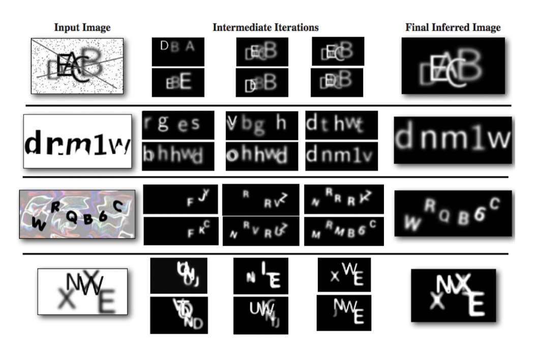
Captcha
Mansinghka, V. K., Kulkarni, T. D., Perov, Y. N., & Tenenbaum, J. (2013). Approximate bayesian image interpretation using generative probabilistic graphics programs. Advances in Neural Information Processing Systems, 26.
Object Tracking
Neiswanger, W., Wood, F., & Xing, E. (2014, April). The dependent Dirichlet process mixture of objects for detection-free tracking and object modeling. In Artificial Intelligence and Statistics (pp. 660-668). PMLR.
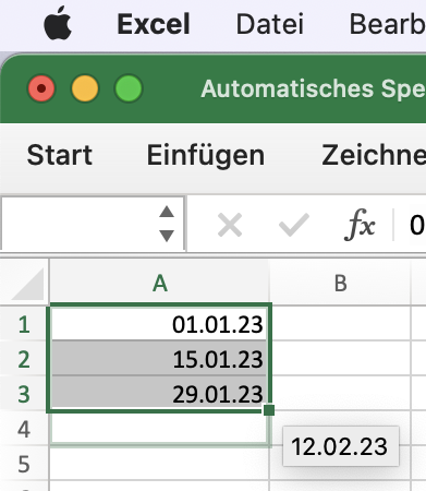
Excel Auto-Fill
Gulwani, S. (2011). Automating string processing in spreadsheets using input-output examples. ACM Sigplan Notices, 46(1), 317-330.
Pose Estimation
Cusumano-Towner, M. F. (2020). Gen: a high-level programming platform for probabilistic inference (Doctoral dissertation, Massachusetts Institute of Technology).
Kulkarni, T. D., Kohli, P., Tenenbaum, J. B., & Mansinghka, V. (2015). Picture: A probabilistic programming language for scene perception. In Proceedings of the ieee conference on computer vision and pattern recognition (pp. 4390-4399).

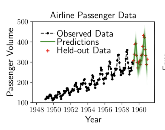
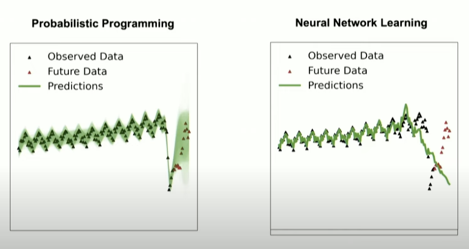
Time Series
Cusumano-Towner, M. F. (2020). Gen: a high-level programming platform for probabilistic inference (Doctoral dissertation, Massachusetts Institute of Technology).
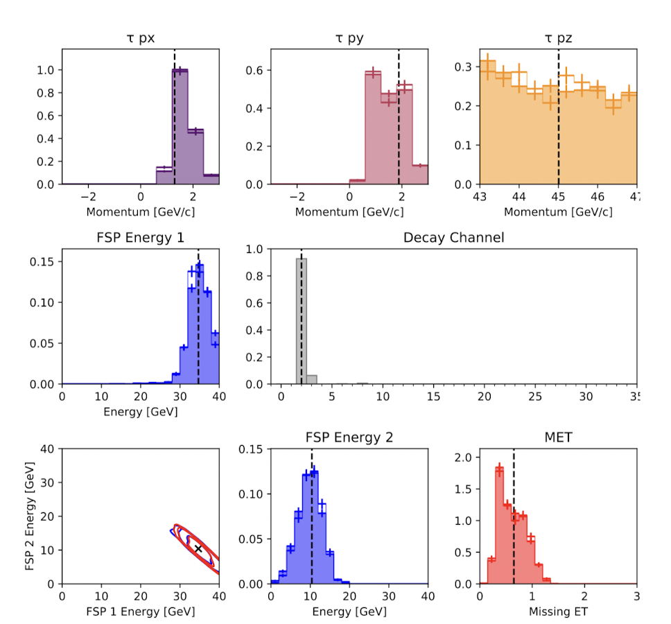
Hadron Collider
Baydin, A. G., Shao, L., Bhimji, W., Heinrich, L., Meadows, L., Liu, J., ... & Wood, F. (2019, November). Etalumis: Bringing probabilistic programming to scientific simulators at scale. In Proceedings of the international conference for high performance computing, networking, storage and analysis (pp. 1-24).
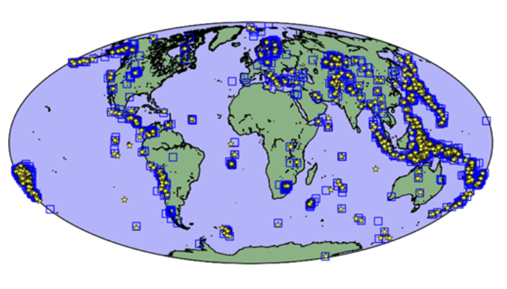
Nuclear Test Detection
Arora, N. S., Russell, S., & Sudderth, E. (2013). NET‐VISA: Network processing vertically integrated seismic analysis. Bulletin of the Seismological Society of America, 103(2A), 709-729.
Further Reading:
- Bayesian Methods for Hackers Probabilistic Programming and Bayesian Inference by Cameron Davidson-Pilon Chapter 1
- https://seeing-theory.brown.edu Chapters 1,2,3,5
- https://youtu.be/HZGCoVF3YvM?si=gw-H4lalEG8tR3PS 3Blue1Brown Bayes Theorem